LRFTubes example: radiation impedance of a baffled piston

© 2018 - ASCEE

This example shows how to use the radiation impedance of a baffled piston as a boundary condition on an acoustic network. See picture below:

# Import necessary stuff
from lrftubes import Air, PrsDuct, System, Z_piston
%pylab inline

Populating the interactive namespace from numpy and matplotlib

# Create a material, with default temperature and pressure
mat = Air()
# Create a system
sys = System(mat)

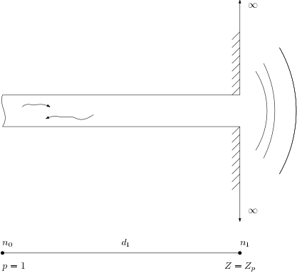
# Dimensions of a simple circular duct
r = 0.1
L = 2.0
S = np.pi*r**2

duct = PrsDuct(L, S, cs='circ')
# Add the duct to the system, set the left node at 0, the right node at 1
sys.addSeg(0, 1, duct)

# Set a unit pressure boundary condition on node 0
sys.addBc('p', 0, 1.0+0j)

# Create the radiation impedance functor
Zp = Z_piston(mat, r)

# Add the radiation impedance functor as impedance boundary condition on the
# right side.
sys.addBc('Z', 1, Zp)

# Create a range of frequencies, solve for these.
f = np.linspace(10, 10000, 500)
sol = sys.solve(f)

# Obtain the pressure and velocity at the impendance b.c. node
pR = sol[duct]['pR']
uR = sol[duct]['UR']/S

# Compute and plot impedance
zr = pR/uR

figure(figsize=(12,6))
semilogx(f,zr.real)
semilogx(f,zr.imag)
title('Real and imaginary part of the radiation impedance of a baffled piston')
xlabel('Frequency [Hz]')
ylabel('Z [rayls]')

legend(['Real part', 'Imaginary part'])

<matplotlib.legend.Legend at 0x7f898fde8cf8>